
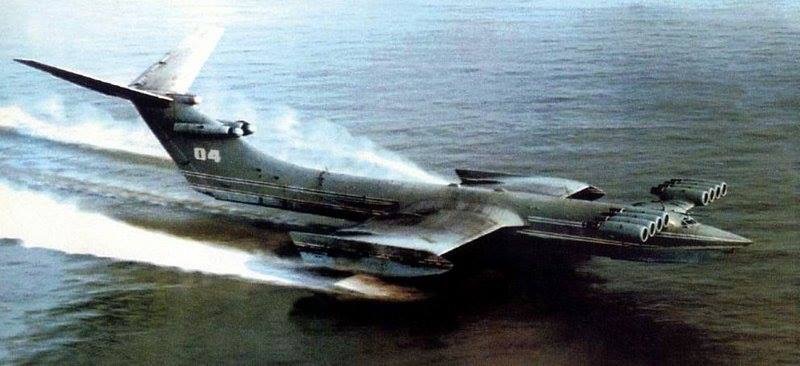
Without doubt, the nation that has progressed ground-effect-vehicles the furthest is Russia. More specifically, this was the USSR from the 1960s through to the late 1980s with their Ekranoplan aircraft. These GEVs (Ground Effect Vehicles) were designed by the Central Hydrofoil Design Bureau, at the heart of the aerodynamic design was the Department of Hydromechanics of the Marine Technical University (DHMTU) in Saint Petersburg.
The DHMTU established an aerofoil series whose geometries are defined analytically, which to my knowledge is the only series of parametrised aerofoils designed specifically for ground effect flight. The definition varies quite significantly from the NACA 4-digit aerofoils, already in GEVfoil. The aerofoil has a partly or fully flat base with an s-shaped mean camber line.
DHMTU Notation
The DHMTU aerofoils notation has eight digits, given as follows:
DHMTU Y1-X1-Y2-X2-Y3-X3-δup-RLE
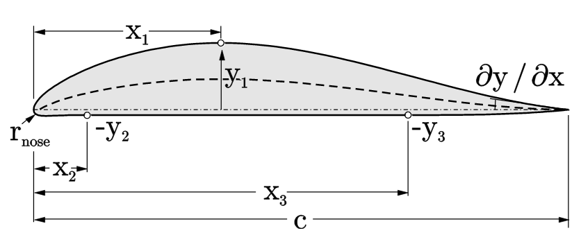
| Y1 | maximum ordinate of the upper surface (%c) |
| X1 | abscissa of Y1 (%c) |
| Y2 | ordinate of the start of the flat section (%c, positive value represents negative y) |
| X2 | abscissa of Y2 (%c) |
| Y3 | ordinate of the end of the flat section (%c, positive value represents negative y) |
| X3 | absissa of Y3 (%c) |
| δup | slope parameter of the upper trailing edge |
| RLE | leading edge radius parameter |
Some DHMTU sections from the literature include DHMTU 12-35-3-10-2-80-12-2 [1] and DHMTU 10-40-2-10-2-60-21-5 [2]. These names don’t exactly register in memory as readily as the likes of the NACA 0012! The JavaFoil manual has a very nice figure of the DHMTU section:
The above information is readily available in some western papers such as Moore’s [1], theses such as a Smuts [2] and manuals such as JavaFoil by Hepperle [3]. However, no further information is given. Moore, from 2002, references a South Korean website, which is now defunct. Hepperle references a Korean document from 1996; ‘Development of S-shaped Section (DHMTU Family)‘ by Chun Ho-Hwan, Chang Chong-Hee of Pusan University. No further information is given about this document, for example whether it’s a conference paper, a journal paper or perhaps a thesis, and despite my best efforts I was initially unable to find this document online.
With thanks to my friends in the Wing In Ground Effect group on groups.io I have managed to obtain the ‘Development of S-shaped Section’ paper in Korean [4] from a member’s personal archive (thank you, Marc!). I cannot recommend this group enough for those with an interest in ground effect craft, it is the successor to the long standing group of the same name on Yahoo Groups, whose service is moribund.
I have absolutely no command of the Korean language, however the equations and diagrams are mutually intelligible, and the online translators are adequate enough. I have done my best to capture this information below. At a future date I will explore options for more formally capturing my findings following some further analysis, in the hope that this fascinating aerofoil family can be recorded for prosperity in western literature.
The following is my best attempt (along with online translators) to understand this document.
Defining the Upper-Surface
The upper-surface is split into a fore and aft section, the fore starting at the leading edge and terminating at the maximum y ordinate, Y1. The aft section somewhat intuitively starts at Y1 and ends at the trailing edge.
Upper-surface – Fore Section
\[ y_{upper} = a_0 \sqrt{x} + a_1 x + a_2 x^2 +a_3 x^3 \]subject to \[0 < x < x_1\]
And secondly the upper-surface aft of the maximum ordinate:
\[ y_{upper} = d_0 + d_1(1-x) + d_2(1-x)^2 + d_3(1-x)^3 \]subject to \[ x_1 < x < 1\]
The parameters a0 to a4 are obtained via a fairly convoluted process.
Leading edge radius \[r_t = a_0/2\]
Leading edge parameter \[ r_{nose} = r / t+u^2\]
Radius at the point X1 is \[R = \frac{1}{(2d_2+6d_3(1-x_1)}\]
The paper then works through some derivation – and it is unclear throughout the paper whether this is the interpretation of the author, or whether this is the author translating from an original and unreferenced Russian document. Four conditions are given as a set of linear equations:
Condition 1 (for a0):
\[t_u = a_0 \sqrt{x_t} + a_1 x_t+a_2 x_t^2+a_3 x_t^3\]
\[t_u – a_0 \sqrt{x_t} = a_1 x_t+a_2 x_t^2+a_3 x_t^3\]
Condition 2 (for a1):
\[y’_{upper}(x=x_t) = \frac{a_0}{2\sqrt{x_t}} + a_1 + 2 a_2 x_t + 3a_3 x_t^3= 0\] \[-\frac{a_0}{2\sqrt{x_t}} = a_1 + 2a_2x_t+3a_3x_t^3\]Condition 3(for a2):
\[r=kt_u^2\] \[k t_u^2 = a_0^2 / 2\] \[\therefore a_0 = \sqrt{2k}t_u\]Condition 4 (for a3):
\[y_{upper} = \frac{1}{R} \] \[2a_2 + 6a_3x_t = 2d_2 + 6d_3(1-x_t) + a_0/4x_t^{\frac{3}{2}}\]Upper-surface – Aft Section
For the aerofoil aft of the maximum ordinate, the four parameters d0 to d3 are obtained via similarly convoluted process.
Condition 1:
\[t_u = d_0 + d_1(1-x_t) + d_2(1-x_t)^2 + d_3(1-x_t)^3\] \[t_u = -\delta_b(1-x_t) + d_2(1-x_t)^2 + d_3(1-x_t)^3\]Condition 2:
\[y_{up} ^ {\prime} = – d_1 + 2d_2(1-x_t) – 3d_3(1-x_t)^2 = \delta_b – 2d_2(1-x_t) -3d_3(1-x_t)^2\] \[2d_2(1-x_t)=\delta_b -3d_3(1-x_t)^2\] \[d_2 = \frac{\delta_b – 3 d_3( 1-x_t)^2}{2(1 – x_t)}\] \[t_u=-\delta_b(1-x_t)+d_2(1-x_t)^2+d_3(1-x_t)^3\] \[=-\delta_b(1-x_t)+\frac{\delta_b-3d_3(1-x_t)^2}{2(1-x_t}(1-x_t)^2+d_3(1-x_t)^3\] \[=-\delta_b(1-x_t)+\frac{1}{2}\delta_b(1-x_t)-\frac{3}{2}d_3(1-x_t)^3+d_3(1-x_t)^3\] \[=\frac{1}{2}\delta_b(1-x_t)-\frac{1}{2}\delta_3(1-x_t)^3\] \[\therefore \frac{1}{2}d_3(1-x_t)^3=–\frac{1}{2}\delta_b(1-x_t)-t_u\] \[d_3 = \frac{-\delta_b(1-x_t)-t_u}{(1-x_t)^2}=\frac{-\delta_b-\frac{t_u}{(1-x_t)}}{(1-x_t)^2}\] \[d_2 = \frac{t_u+\delta_b(1-x_t)-d_3(1-11x_t)^3}{(1-x_t)^2}\]Condition 3:
Mercifully, the third condition simple:
\[ d_0 = 0 \]Condition 4:
\[y_{upper}\prime=-d_1-2d_2(1-x)-3d_3(1-x)^2\] \[\delta_b = -d_1\hspace{0.5cm}at\hspace{0.5cm} x = 1\] \[\therefore d_1 = – \delta_b \]Defining the lower-surface
The lower surface is split into three sections, the curved fore section, similar to the upper-section, a flat mid section and a curved aft section.
Lower-surface – Fore Section
As with the upper-surface:
\[ y_{lower} = b_0 \sqrt{x} + b_1 x + b_2 x^2 +b_3 x^3 \]subject to: \[0 < x < x_1\]
The four parameters a0 to a4 are obtained via a fairly convoluted process.
tlower is the ordinate of the lower surface at point x1.
y” = 0 at point x1.
Leading edge radius:
\[r_t=\frac{b_0^2}{2}\]At the point x1:
\[\frac{dy}{dx}fore =\frac{dy}{dx}mid\]That is to say, there is continuity at the interface of the sections.
Condition 1
\[b_1x_1+b_2x_1^2+b_3x_1^3=t_{lower}-b_0\sqrt{x_1}\]Condition 2
\[2b_2+6b_3x_1=\frac{b_0}{4x_1^{\frac{3}{2}}}\]Condition 3
\[k=\frac{r}{t_u^2}\] \[r=t_u^2k\] \[b_0\sqrt{2kt_u}=a_0\]Condition 4
\[b_1+2b_2x_1+3b_3x_1^2=c_1-b_0 / 2\sqrt{x_1}\]Lower Surface – Mid-Section
The flat middle section is somewhat simply defined, between x1<x<x2:
\[y_{lower} = -c_0 – c_1 (x-x_1)\] \[c_0 =t_{lower}\] \[c_1 = \frac{t_{lower2}-t_{lower}}{x_2-x_1} \]Lower Surface – Aft-Section
Finally, the aft-section is defined in a manner not entirely dissimilar to the fore, between x2 < x < (c=1):
\[y_{lower} = -(e_0+e_1(1-x_t)+e_2(1-x_t)^2+e_3(1-x_t)^3)\]tlower2 is the ordinate of the lower surface at point x2.
y” (x2) = 0 at point x1.
At x=1 y(1)=0 – that is to say the trailing edge is (1, 0), i.e. an abscissa of 1 with an ordinate of zero. Noting that we defining this aerofoil with a normalised chord at unity, as is customary with aerofoils.
At the point x2:
\[\frac{dy}{dx}mid =\frac{dy}{dx}aft\]Once again I believe the paper is just telling us there is continuity and no gradient change at the point where the mid and aft sections meet.
The pattern continues once one with linear expressions and coefficient definition:
Condition 1
\[e_0+e_1(1-x_2)+e_2(1-x_2)^2+e_3(1-x_2)^3 = t_{lower2}\]Condition 2
\[2e_2+6e_3(1-x_2)=0\]Condition 3
\[e_0 = d_0 = 0\]Condition 4
\[e_1-2e_2(1-x_2)-3e_3(1-x_2)^2 = – c_1\]Thoughts and Conclusions
The mathematics behind the DHMTU sections are certainly more complex than other analytically defined geometries such as the well known and used NACA 4-series and 6-series.
It cannot be stressed strongly enough – I have made my best attempt to understand a paper in a foreign language (Korean), I have no understanding as to the validity of said reference. Consequently, I cannot have much confidence in these equations as they are presented.
I do have access to some images of DHMTU sections. My next step will be to implement this series into GEVfoil and attempt to reproduce the shapes, to increase confidence.
[1] Moore, N., Wilson, P.A. and Peters, A.J. (2002) An investigation into wing in ground effect aerofoil geometry. In RTO-MP-095. NATO RTO.
[2] Smuts, E. (2009) A Computational Study of a Lifting Wing in Close Proximity to a Moving Ground Plane. Masters Dissertation.
[3] Hepperle, M (2017). JavaFoil Theory Document. User Manual.
[4] Ho-Hwan, C., Chong-Hee C. (1996). Development of S-shaped Section (DHMTU Family). Unknown publication type.