
Following on from the previous post, on the definition of the DHMTU aerofoil, an initial implementation of this ground-effect specific aerofoil type has been created for GEVfoil. Through the Wing In Ground Effect group on groups.io, a Matlab script was discovered. This Matlab code was created by Martin Hepperl (of JavaFoil [1] fame), in 2012. Thankfully, the Matlab script is open-source, and thus could be translated directly into Python without fear of breaching copyright.
The Python code for this initial translation and implementation has been included at the bottom of this post. Initial attempts to verify the script appear to show that it is working well. Included in the paper from Pusan University [1] is an image of an DHMTU 4-40-1-10-1.5-60-15-3 section. This image was digitised and compared to the same section created by the initial GEVfoil implementation:
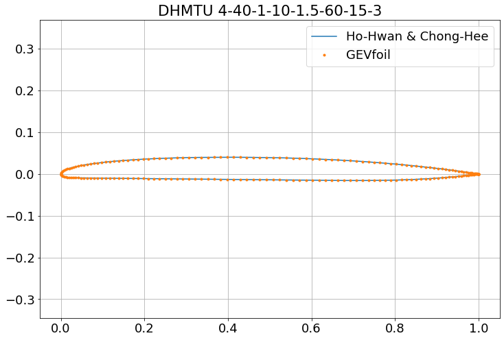
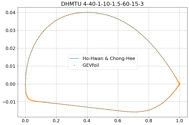
This graph is also redrawn below, with a stretched y-axis, in order to better compare the aerofoil fit, which appears to be excellent. However, it is worth reiterating a point from the previous post, that the validity of this paper is unknown. The author of this blog does not have any definitive original source from the Department of Hydrodynamics at the Marine Technical University (DHMTU), St. Petersburg. It is perhaps unsurprising that these aerofoils match, when both the script is based on the definition from this same source.
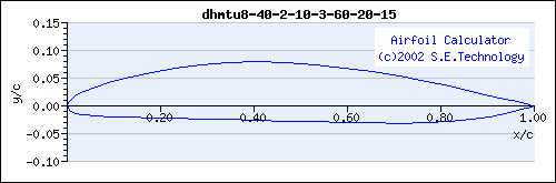
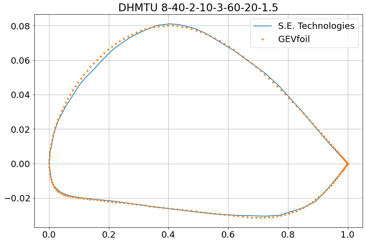
Efforts have been made to find additional DHMTU sections from which to compare. However, the author of this blog post enjoyed limited success due to a lack of these aerofoils in the western literature. This blog’s author has an old, low-resolution image, of a DHMTU 8-40-2-10-3-60-20-1.5, taken via the ‘Airfoil Calculator’ from the now defunct website S.E. Technology.
In spite of the low resolution, best efforts were made to digitise this image, and it was compared against the same section generated in GEVfoil. This comparisons also seems acceptable whilst examined with equal scale spacing:
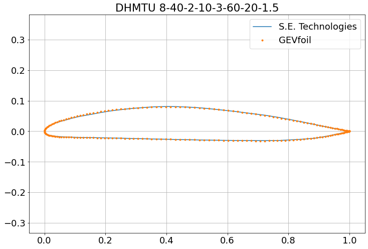
However, when the y-axis is stretched there is some discrepancy, especially around the quarter-chord of the upper-surface, as can be seen in the image below. It is likely that this is simply due to errors introduced in the digitisation of the low-resolution image. Broadly, it can be said that the shape is similar, and there is no reason to distrust the result produced by this initial implementation of DHMTU in GEVfoil.
It is hoped that further examples will be found for comparison. The DHMTU Python implementation, as it stands, is included below. Please note, that unlike the rest of GEVfoil, this script is GNU General Purpose Licence (GPL), as it is based on the GPL Matlab script.
#!/usr/bin/env python3

import numpy as np
import matplotlib.pyplot as plt

"""
##############################################################################
This program is free software: you can redistribute it and/or modify
it under the terms of the GNU General Public License as published by
the Free Software Foundation, either version 3 of the License, or
(at your option) any later version.

This program is distributed in the hope that it will be useful,
but WITHOUT ANY WARRANTY; without even the implied warranty of
MERCHANTABILITY or FITNESS FOR A PARTICULAR PURPOSE.  See the
GNU General Public License for more details.

You should have received a copy of the GNU General Public License
along with this program.  If not, see <https://www.gnu.org/licenses/>.

##############################################################################

A simple script to produce DHMTU aerofoils. This script is based on an
open-source script distributed under the GNU GPL, hence the inclusion of the
licence statements of the original script. This differs from the Creative
Commons Attribution-NonCommercial 3.0 Unported License elsewhere in GEVfoil.

Based on the Matlab of (Martin Hepperle) 2012-02-01 which was
converted from the Mathematica provided by Chang Chong-Hee, 1996

Rewritten into Python in April 2021 (Jason Moller)
@author: glypo (Jason Moller)
"""

class DHMTU(object):
    """A class for generating  DHMTU aerofoils"""
    def __init__(self, foil, points=100, chord=1):
        super(DHMTU, self).__init__()

        tu = foil[0] / 100
        xt = foil[1] / 100
        t1 = foil[2] / 100
        x1 = foil[3] / 100
        t2 = foil[4] / 100
        x2 = foil[5] / 100
        delb = foil[6] / 100
        k = foil[7]

        # Determine coefficients
        c0 = t1
        c1 = (t2-t1)/(x2-x1)

        d1 = delb
        d2 =(-2*delb + 3*tu + 2*delb*xt)/(xt-1)**2
        d3 =(  -delb + 2*tu +   delb*xt)/(xt-1)**3

        a0 = np.sqrt(2)*np.sqrt(k)*tu
        a1 = (3*tu)/xt - (15*np.sqrt(k)*tu)/(4*np.sqrt(2)*np.sqrt(xt)) + d2*xt + 3*d3*xt - 3*d3*xt**2
        a2 = (-2*d2) - (6*d3) - (3*tu)/(xt**2) + (5*np.sqrt(k)*tu)/(2*np.sqrt(2)*xt**(3/2)) + 6*d3*xt
        a3 = -3*d3 + tu/xt**3 - (3*np.sqrt(k)*tu)/(4*np.sqrt(2)*xt**(5/2)) + d2/xt + 3*d3/xt

        b0 = np.sqrt(2)*np.sqrt(k)*tu
        b1 = (-8*t1*x1 - 16*t2*x1 + 15*np.sqrt(2)*np.sqrt(k)*tu*x1**(3/2) + 24*t1*x2 - 15*np.sqrt(2)*np.sqrt(k)*tu*np.sqrt(x1)*x2)/(8* x1*(x2-x1))
        b2 = (5*np.sqrt(k)*tu)/(2*np.sqrt(2)*x1**(3/2)) + (3*t1*x2)/(x1**2*(x1-x2)) + (3*t2)/(x1*x2 - x1**2)
        b3 = (-3*np.sqrt(k)*tu)/(4*np.sqrt(2)*x1**( 5/2)) + (t1*x2-t2*x1)/(x1**3*(x2-x1))

        e1 = (2*t1 - 2*t2 + 3*t2*x1-2*t1*x2 - t2*x2) / (x1-x2-x1*x2 + x2**2);
        e2 = (3*(t2-t1-t2*x1 +t1*x2))/((1-x2)**2*(x1-x2))
        e3 = (t2-t1-t2*x1 +t1*x2)/((x1-x2)*(x2-1)**3)

        # prepare table of points from trailing edge via upper surface to nose and back to trailing edge
        phiRange = np.linspace(np.pi, 0, points)

        xp = np.zeros(2 * points-1)
        yp = np.zeros(2 * points-1)

        # 1-based index of leading edge point
        idxLE = points-1

        for i, phi in enumerate(phiRange):
            x = (1 + np.cos(phi)) / 2

            # upper surface
            if x <= xt:
               yu = a0*np.sqrt(x) + a1*x + a2*x**2 + a3*x**3;
            else:
               yu = d1*(1-x) + d2*(1-x)**2 + d3*(1-x)**3

            xp[idxLE-i] = x
            yp[idxLE-i] = yu

            # lower surface
            if x <= x1:
               yl = -b0*np.sqrt(x) - b1*x -b2*x**2 - b3*x**3
            elif x <= x2:
               yl = -c0 - c1*(x-x1)
            else:
               yl = -e1*(1-x) - e2*(1-x)**2 - e3*(1-x)**3

            xp[idxLE+i] = x
            yp[idxLE+i] = yl

        # Scale the chord
        xp = xp * chord
        yp = yp * chord

        #plt.plot(xp, yp, '.')
        plt.plot(xp, yp)
        plt.grid(True)
        plt.axis('equal')
        plt.show()


if __name__ == "__main__":
    test = DHMTU([12, 35, 3, 10, 2, 80, 12, 2])
In summary, it is believed this initial implementation is working as expected. Thus, it is hoped that this blog’s author can shortly commence some aerodynamic analyses.
[1] Hepperle, M (2017). JavaFoil Theory Document. User Manual.
[2] Ho-Hwan, C., Chong-Hee C. (1996). Development of S-shaped Section (DHMTU Family). Unknown publication type.